Atomsk
The Swiss-army knife of atomic simulations

The Swiss-army knife of atomic simulations


In this tutorial you will learn how to generate unit cells for various lattice types with Atomsk. You will also learn how to generate output files for various visualization softwares. For visualization, it is recommended to install OVITO, Atomeye, XCrySDen, and/or VESTA.
▶ For more information, refer to the corresponding documentation page.
Generating unit cells can be useful to make illustrations, e.g. to explain the basics of crystallography to students or to the public. In atomic-scale simulations, it is often the first step before constructing more complex systems. Atomsk can be used to generate certain types of unit cells, thanks to the mode "--create".
In addition to this tutorial, it is recommended to read the documentation page of the mode "--create".
Many metals, like aluminium, copper, or nickel, crystallize into the fcc lattice.
Let us start with aluminium (symbol Al). Aluminium is a fcc metal with a lattice constant a=4.046 Å at ambiant temperature. To generate a unit cell, Atomsk can be executed like this:
atomsk --create fcc 4.046 Al aluminium.cfg
ⓘ This lattice constant is given as an example, and must be adjusted depending on the type of simulation you want to perform (DFT, interatomic potential, etc.).
With this command, Atomsk will write the atom positions in the output file "aluminium.cfg". It is a text file, and if you open it in a text editor (like Notepad) it will look like this:
Number of particles = 4

              # Fcc Al oriented X=[100] Y=[010] Z=[001].

              A = 1.000000000 Angstrom (basic length-scale)

              H0(1,1) =       4.04600000

              H0(1,2) =       0.00000000

              H0(1,3) =       0.00000000

              H0(2,1) =       0.00000000

              H0(2,2) =       4.04600000

              H0(2,3) =       0.00000000

              H0(3,1) =       0.00000000

              H0(3,2) =       0.00000000

              H0(3,3) =       4.04600000

              .NO_VELOCITY.

              entry_count = 3

                26.9815

              Al

              0.00000000    0.00000000    0.00000000

              0.50000000    0.50000000    0.00000000

              0.00000000    0.50000000    0.50000000

              0.50000000    0.00000000    0.50000000
This file complies with the CFG format, as defined by Ju Li for his visualization software Atomeye. The first line indicates that the system contains 4 atoms. The second line (starting with #) is a comment that is automatically generated by Atomsk. Then appear the vectors of the unit cell (lines starting with H0), followed by some keywords, and finally the atom mass and chemical symbol, and their positions. Note that atom positions are given in reduced coordinates in this file format, i.e. as a fraction of the cell vectors.
Such a file in CFG format can be opened with OVITO, a visualization and analysis software designed by Alexander Stukowski and co-authors, thus allowing to visualize the unit cell in 3-D:
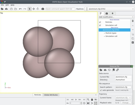
We can see that OVITO displays the Cartesian frame of reference (coloured arrows labeled X, Y, Z at the bottom left corner), the contours of the unit cell (black box), as well as the fours atoms as expected (grey spheres).
Now, let us open the exact same file "aluminium.cfg" with another visualization software, Atomeye:
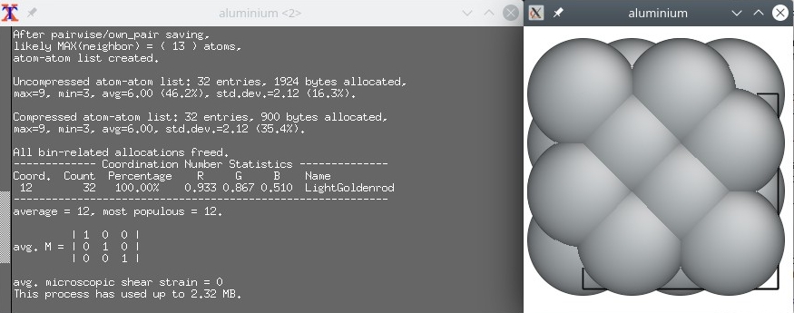
Here we witness a behaviour that is specific to Atomeye. The system is very small (it is only one unit cell), so Atomeye automatically duplicates it twice in each direction. In its terminal it writes that there are "32 atoms" in the system. This is just an artefact of visualization, as we know that there are really only 4 atoms in this system. This is an important lesson to keep in mind: the number of atoms displayed by a visualization software does not always match the actual number of atoms present in the data file.
Now for a change, let us construct a unit cell of copper. Copper (symbol Cu) has an fcc lattice just like aluminium before, so it will also contain 4 atoms, but the lattice constant will be different: a=3.597 Å for copper. This time, let us write the data both in CFG format and in XSF format:
atomsk --create fcc 3.597 Cu copper.cfg xsf
Note that, in addition to the file name "copper.cfg", we added the keyword "xsf" at the end of the command line. This time, Atomsk will generate two output files: "copper.cfg" and "copper.xsf". Let us visualize the first file, "copper.cfg", with OVITO:
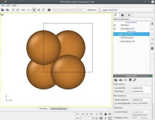
Not much is new here, visualization is pretty similar to the aluminium unit cell above. OVITO uses different colours for atoms of different chemical species: grey for aluminium, orange for copper.
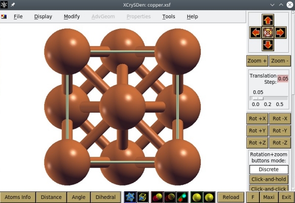
Now let us visualize the second file, "copper.xsf" -which of course contains also 4 atoms. OVITO can also import XSF files, so you can use it to verify that OVITO displays the same figure with both files, CFG and XSF. Now let us try another visualization software. The XSF file format was originally designed by Anton Kokalj for his visualization software XCrySDen, so let us open our file "copper.xsf" with XCrySDen:
Alternatively, XSF files can also be opened with VESTA, as illustrated below:
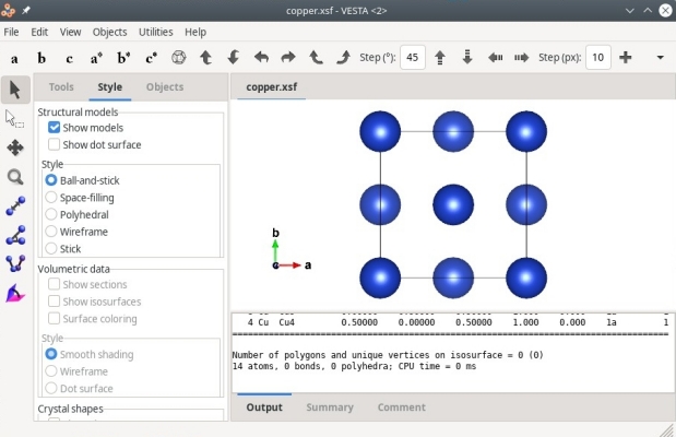
As before we know that there are only 4 atoms in the system, but XCrySDen or VESTA display more atoms than that. This is because these softwares assume periodic boundary conditions, and display the replica of atoms if they belong to the cell. For instance, the first atom of coordinates (0,0,0) appears at each corner of the cell due to periodicity. This is why these softwares display a cell containing 14 atoms. Again, keep in mind that what you see in a visualization software may not correspond to the contents of your data file.
As a second example, let us turn to another lattice type: the body-centered cubic (bcc) lattice. This is the lattice of many transition metals, like iron (Fe) or tungsten (W).
Obviously, in the command-line the parameter "fcc" has to be replaced with "bcc". For example, bcc iron has a lattice parameter 2.856 Å, so one has to use:
atomsk --create bcc 2.856 Fe xsf cfg
In this command-line, we did not specify an output file name. Only output file formats are specified: "xsf" and "cfg". In this situation, Atomsk will use the name of the element (here "Fe") to generate the file name. So, two files will be written by Atomsk: "Fe.cfg" that can be visualized with Atomeye, and "Fe.xsf" that can be opened with XCrySDen.
Similarly, to generate a unit cell of tungsten with lattice constant 3.155 Å:
atomsk --create bcc 3.155 W xsf
Likewise, Atomsk will use the element symbol ("W") to generate the output file name: "W.xsf".
The cubic unit cell of bcc contains two atoms. The files generated above, "Fe.xsf" and "W.xsf", can be opened with VESTA:
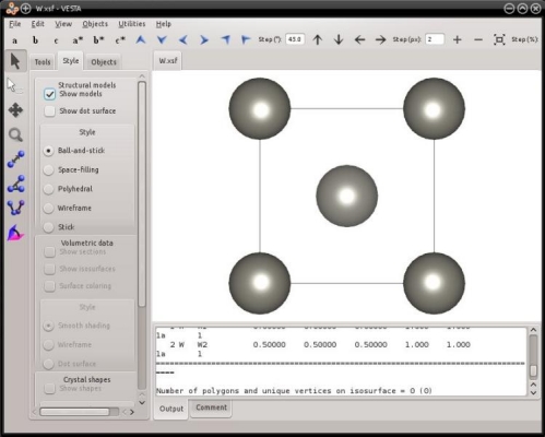
As before, VESTA automatically assumes periodicity, and displays the periodic replica of atoms.
The previous lattice types are quite simple and apply to only one type of atoms. Some lattices can host several chemical species, like the lattice of the table salt: natrium chloride (NaCl) with the rocksalt lattice.
Atomsk can generate this type of lattice with the keyword "rocksalt". After the lattice constant (5.64 Å for NaCl), two chemical symbols have to be provided:
atomsk --create rocksalt 5.64 Na Cl xsf
ⓘ By default, Atomsk generates only the atom positions, and does not assign electric charges to ions. To define electric charges, proceed to this tutorial.
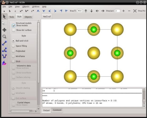
With these instructions Atomsk will construct a unit cell of rocksalt NaCl, and write it into the file "NaCl.xsf", which can be visualized with VESTA:
The mode "--create" is not limited to cubic lattices. One can also generate hexagonal lattices, namely hexagonal close-packed (hcp), wurtzite, or graphite.
Let us create a unit cell of hcp magnesium. Two lattices constants, a and c, must be provided:
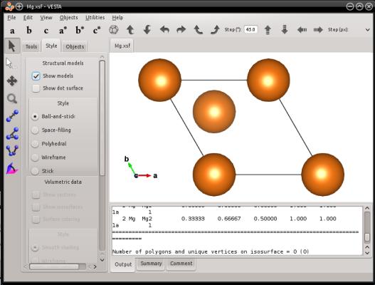
atomsk --create hcp 3.21 5.213 Mg Mg.xsf
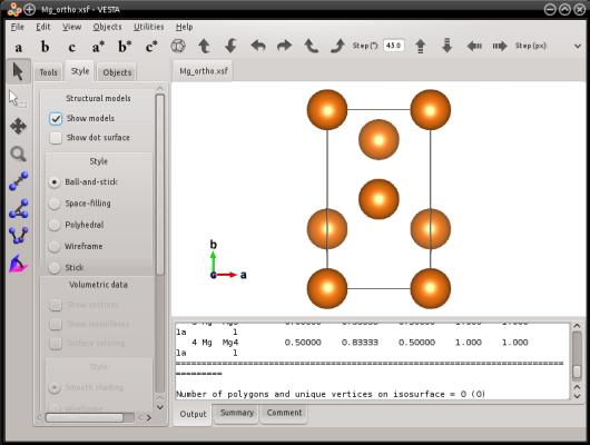
Visualization (here with VESTA) shows that indeed, a unit cell of hcp magnesium was created:
If you wish to obtain an equivalent orthogonal cell (but that still respects the hexagonal lattice), you may use the option "-orthogonal-cell". This option searches for linear combinations of the cell vectors, so as to obtain a rectangular box, and then it fills this new box with atoms. In the case of hcp magnesium, you can use the following command:
atomsk --create hcp 3.21 5.213 Mg -orthogonal-cell Mg.xsf
If you visualize this system, you will see that it is an orthogonal cell of hcp magnesium:
Similarly, Atomsk also allows you to generate a graphite lattice:
atomsk --create graphite 3.21 5.213 C graphite.xsf
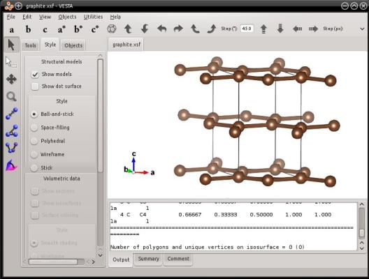
Here, VESTA displays bonds, and displays carbon atoms that are outside of the box. But the text file actually contains just the four atoms of the graphite unit cell, as you can verify by opening it in a text editor.
Atomsk can generate unit cells for various cubic, tetragonal, and hexagonal lattice types. Please read the documentation page to know which types of lattices are supported.
What if I want to create a unit cell that is not supported? Then, the best is to obtain a file describing the structure from another source. In particular, many structures are described in files in the CIF format, which can be obtained from online databases like Crystallography Open Database or the American Mineralogist database. You may also try to enter the name of your material followed by "CIF" in your favorite search engine. This tutorial explains how Atomsk can import CIF files.
Alternatively, if you know the space group and Wickoff positions of the compound, you can use a dedicated software to construct the unit cell. For example, VESTA has a built-in capability for constructing atomic structures (open VESTA, go to File → New structure).
Finally, most of the time a unit cell contains only a few atoms. You may write down the atom positions into a text file, along with the dimensions of the cell. Make sure to write it in a format that Atomsk can read, like the XYZ format (see the list of supported formats). Then, Atomsk can read your file and manipulate the data.
Often, one wants to duplicate the unit cell of the material to generate a larger crystal, called a "supercell". This can be achieved with the option "-duplicate". This option can be used in combination with the mode "--create", for instance the following will create a supercell of tungsten, containing 3 unit cells along X, 4 along Y, and 10 along Z:
atomsk --create bcc 3.155 W -duplicate 3 4 10 xsf
Or, if you already have a file containing a unit cell (or any atomic system), then you may duplicate it:
atomsk initial.xsf -duplicate 3 4 10 final.cfg
ⓘ Those values can be considered as "multiplication factors" along each direction. So, a value of 1 means that the system is multiplied by 1, i.e. its dimension remains unchanged along the given direction ("-duplicate 1 1 1" would cause no change at all). A value of 0 (zero) is automatically replaced by 1, because multiplication by 0 would mean that the system would be completely deleted. Negative values mean that the system is flipped along the given direction.
Duplication always uses the cell vectors as translation vectors, so as to maintain the periodicity of the crystal. So, if your box vectors are not orthogonal or not aligned with Cartesian axes, do not worry: Atomsk does not use Cartesian directions to duplicate, but the vectors of the initial cell, whatever they may be.
As you can see from the previous examples, it is very simple to generate files for visualization with Atomsk. If you have a favorite visualization software, then you may adapt the following tutorials to generate files in a suitable format. For instance if you are familiar with Atomeye or OVITO, then write your data files in the CFG format. If you are more familiar with VESTA or XCrySDen, then use the XSF format.
If you wish to orient the crystal differently, please proceed to the next tutorial.
Now use your imagination! You can change the chemical elements at will. You may also read the documentation of the mode --create and generate unit cells for other types of lattices, and even to create nanotubes.