Atomsk
The Swiss-army knife of atomic simulations

The Swiss-army knife of atomic simulations


This tutorial exposes three methods to construct a ½[110] edge dislocation in aluminium. It is recommended to be familiar with the theory of dislocations in order to follow the steps below.
▶ For more information, refer to the corresponding documentation page.
Aluminium is a face-centered cubic (fcc) metal, where the most favorable slip system is of the type ½⟨110⟩{111}. Assume that we want to construct a system containing only one edge dislocation, lying along the Cartesian Z axis, of Burgers vector b=½[110], in a {111} plane normal to the Y axis, as shown in the schematic illustration below:
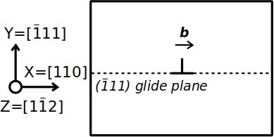
Before anything, we need a unit cell with the crystal orientation that will later allow to introduce the dislocation. Let us use Atomsk to create a unit cell of aluminium with the orientation X=[110] (direction of the Burgers vector b), Y=[111] (normal to the glide plane), Z=[112]:
atomsk --create fcc 4.046 Al orient [110] [-111] [1-12] Al_unitcell.xsf
ⓘ This lattice constant is given as an example, and must be adjusted depending on the type of simulation you want to perform (DFT, interatomic potential, etc.).
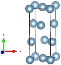
Visualization e.g. with VESTA shows what this unit cell looks like:
To create an atomic system containing a dislocation, we will actually need a supercell. The dislocation is periodic along its line (i.e. along Z), therefore the system will not be duplicated along that direction, i.e. the system will be pseudo 2-D:
atomsk Al_unitcell.xsf -duplicate 60 20 1 Al_supercell.xsf
Based on the lattice parameter chosen above, the Burgers vector ½[110] has a magnitude |b|=a/√2=2.860954 Å. Naturally, if you work with a different lattice parameter, then you have to compute the magnitude of the Burgers vector.
ⓘ The value of the Burgers vector must be given accurately, and must be consistent with the lattice parameter of your crystal. Atomsk will not "automagically" adjust this value.
Now, there exist four different ways to construct an edge dislocation with Atomsk:
These methods are explained in more detail below. Each of them has advantages and pitfalls. No method is universally "better" than the others, it all depends on what you want to achieve.
As a first possible method, Atomsk can introduce an edge dislocation while maintaining the number of atoms constant. This is done by using the option "-dislocation" followed by the position of the dislocation in the XY plane (here it is located at the center of the box), the keyword "edge", the line direction (Z), the normal to the glide plane (Y), the magnitude of the Burgers vector, and the Poisson ratio of the material (for aluminium we use ν=0.33):
atomsk Al_supercell.xsf -dislocation 0.51*box 0.51*box edge Z Y 2.860954 0.33 Al_edge.cfg
ⓘ The position of the dislocation can be given as fraction of the box vectors like above ("0.51*box"), or directly in Angströms. The given position should not correspond exactly to an atom position, otherwise that atom would have an infinite displacement. If you obtain strange results like discontinuities, holes or large displacements, then change the position of the dislocation.
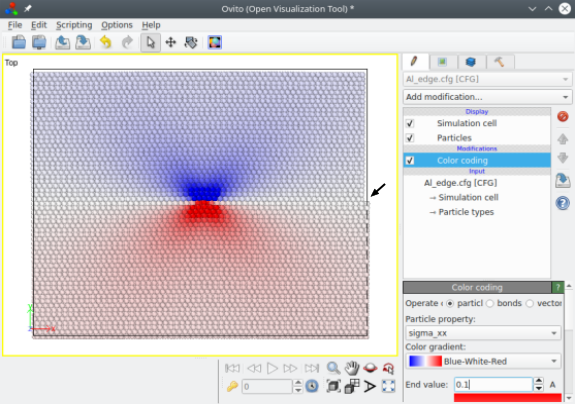
In this case, the upper part of the crystal is compressed, which produces a step on the right-hand border, as it can be seen when opening the file with OVITO (see arrow in the image below). Atomsk also computes the theoretical stress components (from elasticity theory). If you wish to save them, make sure that the final output file supports auxiliary properties, like the CFG format used here; otherwise auxiliary properties are lost. The image below shows the stress component σxx, illustrating the compressive zone above the glide plane (in blue) and the tensile zone below it (in red):
With this method the periodicity of the crystal is lost along both the X and Y directions, which has two consequences. First, performing a simulation will require to "freeze" atoms at the edges of the box (i.e. forbid them to move during relaxation or molecular dynamics), otherwise spurious defects may appear at the borders. Second, if the dislocation moves in its glide plane, it will quickly encounter those frozen atoms, thus preventing its propagation.
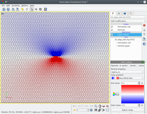
Another possibility is to construct the edge dislocation by inserting a new half-plane of atoms above the glide plane. With Atomsk it can be achieved simply by replacing the keyword "edge" by "edge_add":
atomsk Al_supercell.xsf -dislocation 0.51*box 0.51*box edge_add Z Y 2.860954 0.33 Al_edge_add.cfg
This time, there is no step at the border of the cell. However, because new atoms were introduced the system has grown along the X axis. If periodic boundary conditions are applied, atoms going out of the cell will overlap with other atoms. To prevent that, Atomsk elongates the box vector along X by b/2.
Like before, the periodicity of the system is lost along both the X and Y directions. Another drawback is that it introduces new atoms that did not exist in the initial supercell, making more difficult the comparison with the reference system ("Al_supercell.xsf").
Yet another possibility is to remove a half-plane of atoms below the glide plane. With Atomsk it can be achieved by using the keyword "edge_rm":
atomsk Al_supercell.xsf -dislocation 0.51*box 0.51*box edge_rm Z Y 2.860954 0.33 Al_edge_rm.cfg
Like the previous method, no step is formed at the border of the cell. However, because atoms were removed the system has shortened along the X axis. Atomsk compensates for this by shortening the box vector along X by b/2.
The previous methods have a major drawback: the system is not periodic along the direction of glide of the dislocation (i.e. along X), hence they do not allow to study the glide of a single dislocation. In order to construct a periodic system, another method exists: superimpose two crystals, the top one containing one atomic column in excess compared to the bottom one and being compressed by b/2, and the bottom one being elongated by b/2 so they both have the same length along X.
First, let us construct the two blocks. The bottom block has N=40 columns of atoms, and is elongated by half a unit cell along X, i.e. 0.5/40=0.0125:
atomsk Al_unitcell.xsf -duplicate 40 10 1 -deform X 0.0125 0.0 bottom.xsf
Here we use the option "-deform" with a Poisson ratio of zero, i.e. it is pure tensile strain. Similarly, the top crystal is constructed with N+1=41 atomic columns, compressed along X by 0.5/41=0.012195122:
atomsk Al_unitcell.xsf -duplicate 41 10 1 -deform X -0.012195122 0.0 top.xsf
Then, the mode "--merge" can be used to superimpose the two crystals along Y:
atomsk --merge Y 2 bottom.xsf top.xsf Al_edge_bicrystal.cfg
The final system ("Al_edge_bicrystal.cfg") does not contain a dislocation yet. It only contains two crystals with an increasing mismatch along the X direction, as can be visualized with OVITO (here atoms are coloured according to the centrosymmetry parameter):
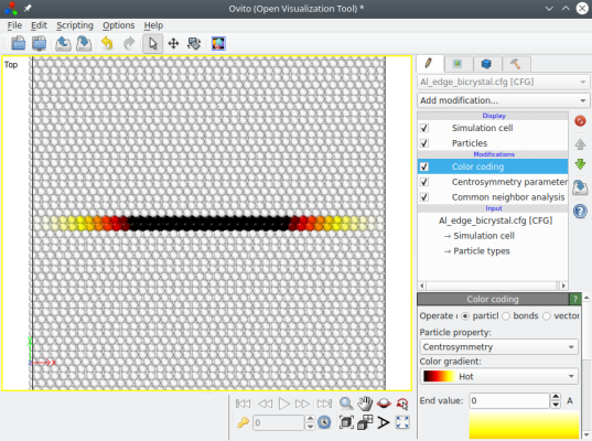
This system is far from equilibrium, and only after a simulation will it relax into an edge dislocation. The advantage of this construction is that it is periodic along the X direction, which makes it suitable for applying a shear stress and studying the motion of the dislocation. However, this system is still not periodic along the Y direction, and it may be necessary to freeze atoms at the top and bottom borders.
It is possible to introduce several edge dislocations in the system. To achieve that, simply call the option "-dislocation" several times, modifying the position and the Burgers vector as needed.
For example, the following command introduces two edge dislocations of opposite Burgers vectors, one at the reduced coordinate (¼ ¼) and the other at (¾ ¾):
atomsk Al_supercell.xsf -dislocation 0.251*box 0.251*box edge_add Z Y 2.860954 0.33 \
-dislocation 0.75*box 0.751*box edge_add Z Y -2.860954 0.33 Al_edge_dipole.cfg
When several dislocations are introduced, their contributions to the stress are summed up, as can be visualized:
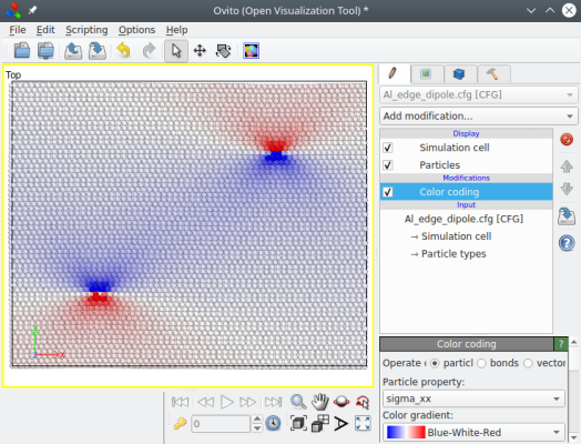
The advantage of a dipole (or quadrupole) is that the sum of the Burgers vectors is zero, hence at long-range the combined elastic field of all dislocations cancel out. As a result, no artefact should appear at the borders, and the system is fully 3-D periodic.
The dislocations constructed with any of the methods above are not relaxed nor optimized. They correspond, at best, to the displacement fields predicted by the elastic theory of dislocations. However, in order to find the actual atomic configuration of the dislocation, the system needs to be optimized (e.g. by performing ab initio or atomistic simulations). For example, in the case of aluminium, it is expected that the ½[110] edge dislocation dissociates into two Shockley partial dislocations. Depending on the method chosen above, the dislocation interacts with frozen boundaries or with other dislocations, which can cause undesirable effects when performing a simulation. You may have to test different system sizes and different dislocation positions to make sure that your results are sound.
While this tutorial focuses on dislocations of pure edge character, it is also possible to construct dislocations of pure screw character with Atomsk, as explained in this tutorial.
By default the option "-dislocation" uses the displacement fields of isotropic elasticity. This is justified in the case of aluminium because it is an isotropic material. In materials that are highly anisotropic, it is recommended to use the anisotropic elasticity to introduce dislocations, as explained in the following tutorial.