Atomsk
The Swiss-army knife of atomic simulations

The Swiss-army knife of atomic simulations


This tutorial explains how to use Atomsk to create a system containing a dislocation and a spherical inclusion, with the example of a spherical silicon inclusion in an aluminium matrix.
Let us begin with the construction of the fcc aluminium matrix. For the sake of simplicity, we will insert the same type of screw dislocation as in a previous tutorial -refer to this tutorial to know more about this dislocation.
Contrary to the previous tutorial where the system contained only a dislocation, here the system should be large enough to contain also a spherical inclusion. In other words it has to be 3-D. The dislocation is placed at (X=0.25,Y=0.5), and the sphere at (X=0.75,Y=0.5) with a radius of 20 Å.
This can be achieved with a single command-line:
atomsk --create fcc 4.046 Al orient [1-12] [-111] [110] \
-duplicate 50 30 30 \
-dislocation 0.251*box 0.501*box screw Z Y 2.860954 \
-select in sphere 0.75*box 0.5*box 0.5*box 20 \
-remove-atoms select \
fccAl_matrix.cfg
Here is the meaning of this command: a unit cell of oriented fcc aluminium is created (with the mode "--create"), then it is duplicated to form a 50x30x30 supercell, then the dislocation is inserted, then a sphere is selected and atoms inside that sphere are removed.
The final system ("fccAl_matrix.cfg") is quite large, it contains about 270,000 atoms. It be visualized with Atomeye:
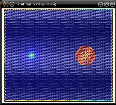
Naturally, because of the screw dislocation, boundary conditions along X and Y are not periodic anymore.
For now, there is just a spherical hole in the aluminium system. Now, let us construct a sphere of silicon. This sphere must be placed at the exact same location as the sphere we carved in aluminium. Atomsk should have displayed the position of the sphere in Å when you ran the previous command: it should be (185.824,105.118,42.914). This position may also be calculated manually, e.g. along X the lattice vector is 1/2[112], of length 4.046*√6/2=9.91063, and we duplicated the cell 50 times, giving a total length of 247.7658. The sphere is placed at 0.75 times this length, i.e. X=185.824. Similarly the Cartesian position of the sphere can be calculated along Y and Z.
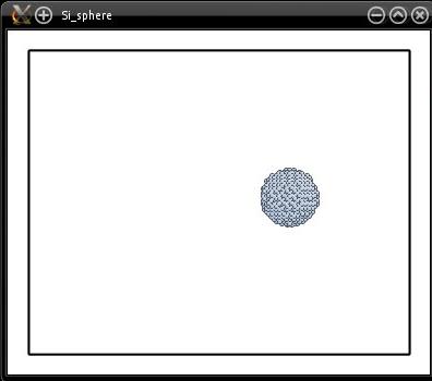
The most simple way to construct the silicon sphere is to create a very large supercell of silicon (at least as large as the aluminium system), and then carve the silicon sphere into it. Note that now, we must select atoms that are outside of the sphere:
atomsk --create diamond 5.431 Si \
-duplicate 60 40 40 \
-select out sphere 185.824 105.118 42.914 20 \
-remove-atoms select \
Si_sphere.cfg
Visualization shows that the sphere looks to be in the right place:
The drawback of this method is that we create a huge box filled with silicon atoms, while only a small sphere of radius 20 Å is needed. In other words, it wastes a lot of memory, and in the end most atoms are deleted. An alternative is to construct a smaller system, just the size of the silicon sphere, and then to displace the sphere to its appropriate coordinates:
atomsk --create diamond 5.431 Si \
-duplicate 10 10 10 \
-shift -0.5*box -0.5*box -0.5*box \
-select out sphere 0 0 0 20 \
-remove-atoms select \
-select none \
-shift 185.824 105.118 42.914 \
Si_sphere.cfg xsf
This method is best illustrated by the schematics below:
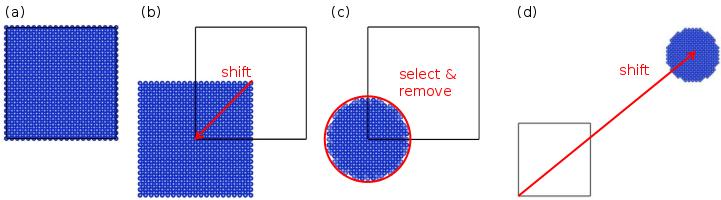
(a) A unit cell of silicon is created and duplicated to form a supercell. The box appears as thick black lines.
(b) Atoms are shifted by (-0.5,-0.5,-0.5). As a result, some atoms are outside of the box.
(c) A sphere of radius 20 Å is selected around the origin (0,0,0). Atoms outside of that sphere are removed.
(d) The sphere is shifted to the desired final position (in this picture the distances are not respected).
If you try to visualize the final system, with most visualization softwares (like Atomeye or VESTA) you will see parts of a sphere inside a box. This is because these visualization softwares automatically wrap the atoms so that they all appear to be inside the box. So what you see is not the actual Cartesian coordinates, but the coordinates shifted so that all atoms are inside the box. Such visualization can be misleading.
Now we just have to merge the two systems:
atomsk --merge 2 fccAl_matrix.cfg Si_sphere.cfg AlSi_final.cfg
The number "2" means that two systems are merged (which names follow). When merging several systems into the same box, the final box is exactly the same as the box of the first system provided. So here, only the box dimensions of the system "fccAl_matric.cfg" are used to define the dimensions of the final box. The box of the silicon system is not used. For that reason, it does not matter which of the two methods above you used to construct the sphere of silicon -the only thing that matters is that you got the Cartesian positions of atoms right.
The final result is written in the file "AlSi_final.cfg", and its visualization shows the dislocation line and the spherical inclusion (atoms in a perfect environment are omitted to facilitate the visualization):
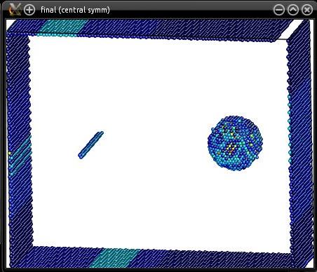
As in a previous tutorial, the screw dislocation that was inserted is not fully relaxed. Also, it is possible to restore the periodicity along the X direction by modifying appropriately the vectors of the final box. This can be useful if one wished to apply stress to move the dislocation and see how it interacts with the inclusion.
The silicon sphere was not created with any specific orientation -it is just oriented X=[100], Y=[010], Z=[001]. Naturally, when creating it it is possible to give it another crystal orientation. It is also possible to give it another radius, or another shape -for instance, instead of selecting a sphere, select atoms in a box.