Atomsk
The Swiss-army knife of atomic simulations

The Swiss-army knife of atomic simulations


This tutorial explains how to compute a radial distribution function (RDF) with Atomsk.
▶ For more information, refer to the corresponding documentation page.
ⓘ Construction of the neighbour list is quite slow in Atomsk up to version beta 0.11.2. For improved performance, use version beta 0.12 or later.
The radial distribution function, or RDF for short, often noted g(r), is a measure of the average density around atoms. If you are not familiar with this concept, you may read the Wikipedia page.
Let us begin with the very simple example of a unit cell of aluminium. Let us construct this cell:
atomsk --create fcc 4.056 Al Al_unitcell.cfg
Then create a text file named "list.txt" with a text editor (like gedit, emacs, vi or similar), and write inside the name of the file to analyze, "Al_unitcell.cfg":
Al_unitcell.cfg
To save time, you may also generate the file "list.txt" with the following command (on UNIX/Linux systems):
ls Al_unitcell.cfg > list.txt
We are now ready to compute the RDF. Atomsk requires the name of the list file, then the maximum distance and the skin width. For example, to compute the RDF up to a distance of 12 Å, using a skin (or sample width) of 0.1 Å:
atomsk --rdf list.txt 12 0.1
ⓘ Instead of "list.txt", you may choose any name you want for the list file. Just make sure to use the matching file name when running the mode "--rdf".
Atomsk writes the RDF in a file named "rdf_total.dat", which we can visualize with a plotting software like xmgrace, gnuplot, or any software of your liking:
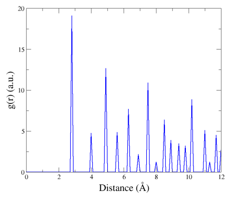
Here the first peak at 2.86 Å corresponds to the distance between first neighbours in the fcc lattice (i.e. a0/√2), the second peak corresponds to second neighbours (a0), and so on.
Notice that although the unit cell is very small (a cube of side 4.046 Å), Atomsk is able to compute the RDF up to much larger distances. This is because periodic boundary conditions are always assumed when computing the RDF, so an atom can have its multiple periodic replicas as neighbours.
Now let us compute the RDF in a larger system, where atoms are randomly displaced:
atomsk Al_unitcell.cfg -duplicate 20 20 20 -disturb 0.2 Al.cfg
Write the name of the file "Al.cfg" into a text file, and then run Atomsk in mode "--rdf":
ls Al.cfg > list.txt
atomsk --rdf list.txt 12 0.1 -wrap
ⓘ Because atoms were displaced, some of them may end up out of the box. We use the option "-wrap" to make sure all atoms are placed back into the box. This is required to correctly build the neighbour list. If you don't use "-wrap" Atomsk will ask you if you wish to wrap atoms. Note that if you refuse, the neighbour list may be wrong, therefore the RDF may also be wrong.
The RDF then looks like the following:
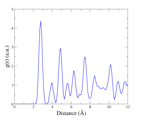
We can see that the peaks are broadened, because atoms were slightly displaced out of their respective lattice sites. Because of this disorder, at long range the RDF tends towards 1.
After performing molecular dynamics (MD), it is sometimes desirable to compute the RDF and average it over several snapshots. Performing actual MD is out of the scope of this tutorial, so let us just construct several configurations with Atomsk, by displacing atoms randomly, for instance with these three commands:
atomsk Al_unitcell.cfg -duplicate 20 20 20 -disturb 0.2 Al_1.cfg
atomsk Al_unitcell.cfg -duplicate 20 20 20 -disturb 0.2 Al_2.cfg
atomsk Al_unitcell.cfg -duplicate 20 20 20 -disturb 0.2 Al_3.cfg
Let us pretend that these configurations are "snapshots" from a MD run. All we have to do, is write all their file names into a list file, and run Atomsk in mode "--rdf":
ls Al_[1-3].cfg > list.txt
atomsk --rdf list.txt 12 0.1 -wrap
ⓘ Options (like the option "-wrap" used here) are applied to each system before computing its RDF.
Atomsk will compute the RDF for each file, and then compute the average over all configurations. If the configurations are actual snapshots from a MD simulation taken at different times, then you will obtain the time-averaged RDF.
The examples above used fcc aluminium as an example, which contained only one type of atom. Let us now construct a system containing several types of atoms, for instance MgO with the rock-salt structure:
atomsk --create rocksalt 4.2 Mg O -duplicate 10 10 10 -disturb 0.2 MgO.cfg
As before, let us write the name of this file into a list file, and run the mode "--rdf":
ls MgO.cfg > list.txt
atomsk --rdf list.txt 12 0.1 -wrap
You will see that Atomsk produces four files, containing the partial RDF for each pair of type of atoms, and the total RDF:
ⓘ Note that the RDF for the Mg-O pairs is identical to the RDF for the O-Mg pairs, therefore Atomsk only computes the former and not the latter.
You may visualize each of these plots individually, or all together on the same plot:
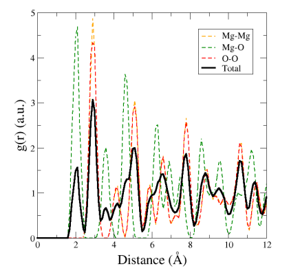
The first peak (green dashed line) corresponds to the Mg-O first neighbour distance. The second peak (orange and red dashed curves) corresponds to second neighbours, and is located at the same distance for Mg-Mg and O-O. This is typical of the rock-salt lattice. Again, peaks are quite broad because we shuffled atoms with the option "-disturb".
As an exercise, you may use Atomsk to construct a cell of perovskite material, which contains three different types of atoms, and then compute its RDF. You will see that Atomsk produces one RDF file for each possible pair of atoms, as well as the total RDF.
Computation of the RDF is quite fast for small systems, like in the examples above. In larger systems it is expected to become slower, mainly because the neighbour search algorithm currently implemented in Atomsk is O(N2). In other words, its running time increases as the square of the number of atoms: doubling the number of atoms will multiply by four the time to construct the neighbour list. Furthermore, increasing the maximum radius R, or the skin size dR, will also increase the time to compute the RDF.